Priority Queues with Binary Heaps

One important variation of the queue is the priority queue. A priority queue acts like a queue in that items remain in it for some time before being dequeued. However, in a priority queue the logical order of items inside a queue is determined by their “priority”. Specifically, the highest priority items are retrieved from the queue ahead of lower priority items.

We will see that the priority queue is a useful data structure for specific algorithms such as Dijkstra’s shortest path algorithm. More generally though, priority queues are useful enough that you may have encountered one already: message queues or tasks queues for instance typically prioritize some items over others.

You can probably think of a couple of easy ways to implement a priority queue using sorting functions and arrays or lists. However, sorting a list is $O(n \log{n})$. We can do better.

The classic way to implement a priority queue is using a data structure called a binary heap. A binary heap will allow us to enqueue or dequeue items in $O(\log{n})$.

The binary heap is interesting to study because when we diagram the heap it looks a lot like a tree, but when we implement it we use only a single dynamic array (such as a Python list) as its internal representation. The binary heap has two common variations: the min heap, in which the smallest key is always at the front, and the max heap, in which the largest key value is always at the front. In this section we will implement the min heap, but the max heap is implemented in the same way.

The basic operations we will implement for our binary heap are:

• BinaryHeap() creates a new, empty, binary heap.
• insert(k) adds a new item to the heap.
• find_min() returns the item with the minimum key value, leaving item in the heap.
• del_min() returns the item with the minimum key value, removing the item from the heap.
• is_empty() returns true if the heap is empty, false otherwise.
• size() returns the number of items in the heap.
• build_heap(list) builds a new heap from a list of keys.

The Structure Property

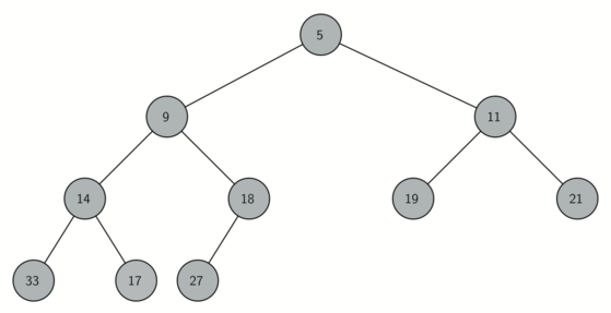
In order for our heap to work efficiently, we will take advantage of the logarithmic nature of the binary tree to represent our heap. In order to guarantee logarithmic performance, we must keep our tree balanced. A balanced binary tree has roughly the same number of nodes in the left and right subtrees of the root. In our heap implementation we keep the tree balanced by creating a complete binary tree. A complete binary tree is a tree in which each level has all of its nodes. The exception to this is the bottom level of the tree, which we fill in from left to right. This diagram shows an example of a complete binary tree:

Another interesting property of a complete tree is that we can represent it using a single list. We do not need to use nodes and references or even lists of lists. Because the tree is complete, the left child of a parent (at position $p$) is the node that is found in position $2p$ in the list. Similarly, the right child of the parent is at position $2p + 1$ in the list. To find the parent of any node in the tree, we can simply use integer division (like normal mathematical division except we discard the remainder). Given that a node is at position $n$ in the list, the parent is at position $n/2$.

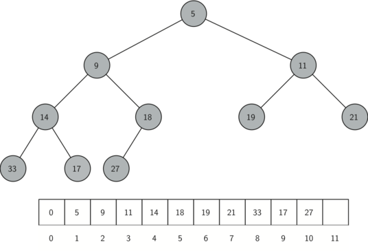
The diagram below shows a complete binary tree and also gives the list representation of the tree. Note the $2p$ and $2p+1$ relationship between parent and children. The list representation of the tree, along with the full structure property, allows us to efficiently traverse a complete binary tree using only a few simple mathematical operations. We will see that this also leads to an efficient implementation of our binary heap.

The Heap Order Property

The method that we will use to store items in a heap relies on maintaining the heap order property. The heap order property is as follows: In a heap, for every node $x$ with parent $p$, the key in $p$ is smaller than or equal to the key in $x$. The diagram below also illustrates a complete binary tree that has the heap order property.

Heap Operations

We will begin our implementation of a binary heap with the constructor. Since the entire binary heap can be represented by a single list, all the constructor will do is initialize the list and an attribute current_size to keep track of the current size of the heap. The code below shows the Python code for the constructor. You will notice that an empty binary heap has a single zero as the first element of items and that this zero is not used, but is there so that simple integer division can be used in later steps.

class BinaryHeap(object):
    def __init__(self):
        self.items = [0]

    def __len__(self):
        return len(self.items) - 1

    

The next method we will implement is insert. The easiest, and most efficient, way to add an item to a list is to simply append the item to the end of the list. The good news about appending is that it guarantees that we will maintain the complete tree property. The bad news about appending is that we will very likely violate the heap structure property. However, it is possible to write a method that will allow us to regain the heap structure property by comparing the newly added item with its parent. If the newly added item is less than its parent, then we can swap the item with its parent. The diagram below shows the series of swaps needed to percolate the newly added item up to its proper position in the tree.

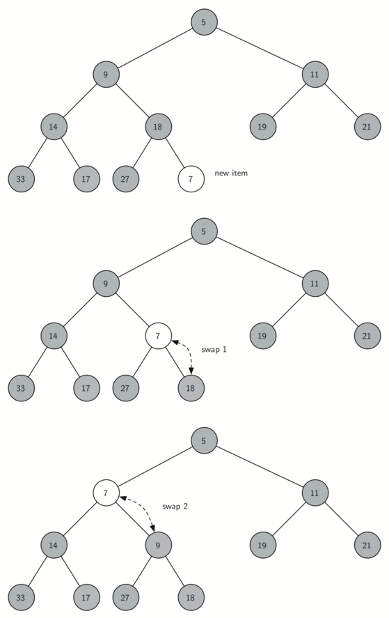
Notice that when we percolate an item up, we are restoring the heap property between the newly added item and the parent. We are also preserving the heap property for any siblings. Of course, if the newly added item is very small, we may still need to swap it up another level. In fact, we may need to keep swapping until we get to the top of the tree. The code below shows the percolate_up method, which percolates a new item as far up in the tree as it needs to go to maintain the heap property. Here is where our wasted element in items is important. Notice that we can compute the parent of any node by using simple integer division. The parent of the current node can be computed by dividing the index of the current node by 2.

    def percolate_up(self):
        i = len(self)
        while i // 2 > 0:
            if self.items[i] < self.items[i // 2]:
                self.items[i // 2], self.items[i] = \
                    self.items[i], self.items[i // 2]
            i = i // 2
    

We are now ready to write the insert method (see below). Most of the work in the insert method is really done by percolate_up. Once a new item is appended to the tree, percolate_up takes over and positions the new item properly.

    def insert(self, k):
        self.items.append(k)
        self.percolate_up()
    

With the insert method properly defined, we can now look at the delete_min method. Since the heap property requires that the root of the tree be the smallest item in the tree, finding the minimum item is easy. The hard part of delete_min is restoring full compliance with the heap structure and heap order properties after the root has been removed. We can restore our heap in two steps. First, we will restore the root item by taking the last item in the list and moving it to the root position. Moving the last item maintains our heap structure property. However, we have probably destroyed the heap order property of our binary heap. Second, we will restore the heap order property by pushing the new root node down the tree to its proper position. The diagram shows the series of swaps needed to move the new root node to its proper position in the heap.

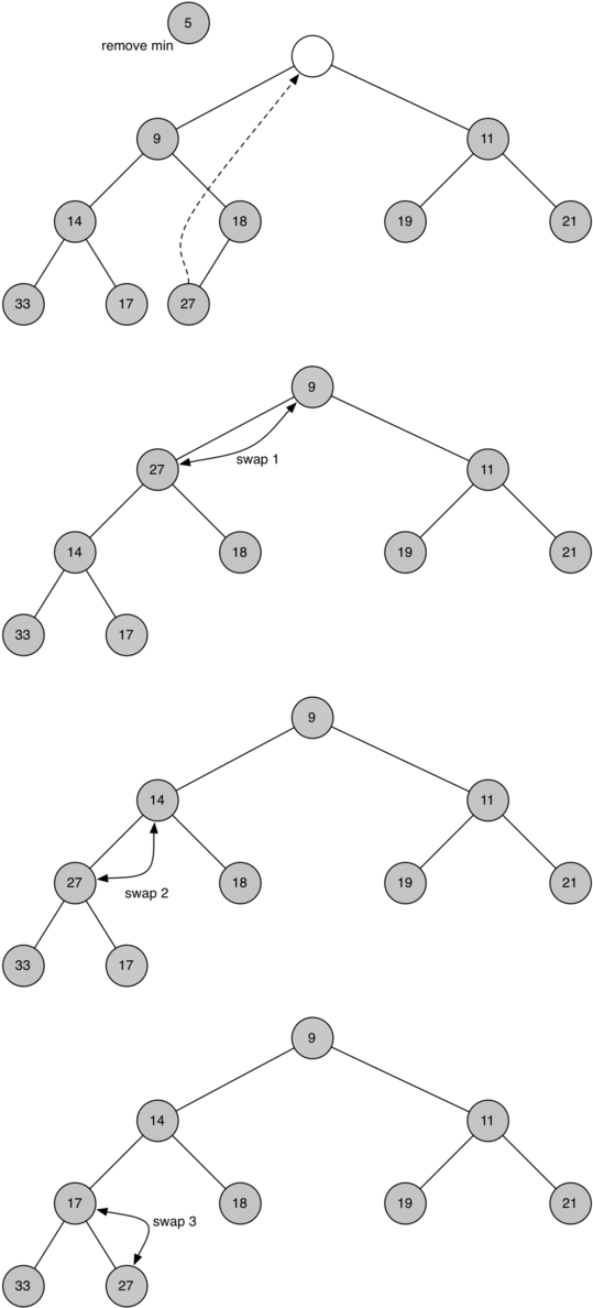
In order to maintain the heap order property, all we need to do is swap the root with its smallest child less than the root. After the initial swap, we may repeat the swapping process with a node and its children until the node is swapped into a position on the tree where it is already less than both children. The code for percolating a node down the tree is found in the percolate_down and min_child methods below.

    def percolate_down(self, i):
        while i * 2 <= len(self):
            mc = self.min_child(i)
            if self.items[i] > self.items[mc]:
                self.items[i], self.items[mc] = self.items[mc], self.items[i]
            i = mc

    def min_child(self, i):
        if i * 2 + 1 > len(self):
            return i * 2

        if self.items[i * 2] < self.items[i * 2 + 1]:
            return i * 2

        return i * 2 + 1
    

The code for the delete_min operation is below. Note that once again the hard work is handled by a helper function, in this case percolate_down.

    def delete_min(self):
        return_value = self.items[1]
        self.items[1] = self.items[len(self)]
        self.items.pop()
        self.percolate_down(1)
        return return_value
    

To finish our discussion of binary heaps, we will look at a method to build an entire heap from a list of keys. The first method you might think of may be like the following. Given a list of keys, you could easily build a heap by inserting each key one at a time. Since you are starting with a list of one item, the list is sorted and you could use binary search to find the right position to insert the next key at a cost of approximately $O(\log{n})$ operations. However, remember that inserting an item in the middle of the list may require $O(n)$ operations to shift the rest of the list over to make room for the new key. Therefore, to insert $n$ keys into the heap would require a total of $O(n \log{n})$ operations. However, if we start with an entire list then we can build the whole heap in $O(n)$ operations. The code below shows the code to build the entire heap.

    def build_heap(self, alist):
        i = len(alist) // 2
        self.items = [0] + alist
        while i > 0:
            self.percolate_down(i)
            i = i - 1

Above we see the swaps that the build_heap method makes as it moves the nodes in an initial tree of [9, 6, 5, 2, 3] into their proper positions. Although we start out in the middle of the tree and work our way back toward the root, the percolate_down method ensures that the largest child is always moved down the tree. Because the heap is a complete binary tree, any nodes past the halfway point will be leaves and therefore have no children. Notice that when i==1, we are percolating down from the root of the tree, so this may require multiple swaps. As you can see in the rightmost two trees of above, first the 9 is moved out of the root position, but after 9 is moved down one level in the tree, percolate_down ensures that we check the next set of children farther down in the tree to ensure that it is pushed as low as it can go. In this case it results in a second swap with 3. Now that 9 has been moved to the lowest level of the tree, no further swapping can be done. It is useful to compare the list representation of this series of swaps as shown in above with the tree representation.

i = 2  [0, 9, 5, 6, 2, 3]
i = 1  [0, 9, 2, 6, 5, 3]
i = 0  [0, 2, 3, 6, 5, 9]

The assertion that we can build the heap in $O(n)$ may seem a bit mysterious at first, and a proof is beyond the scope of this book. However, the key to understanding that you can build the heap in $O(n)$ is to remember that the $\log{n}$ factor is derived from the height of the tree. For most of the work in build_heap, the tree is shorter than $\log{n}$.