General Depth First Search

The knight’s tour is a special case of a depth first search where the goal is to create the deepest depth first tree, without any branches. The more general depth first search is actually easier. Its goal is to search as deeply as possible, connecting as many nodes in the graph as possible and branching where necessary.

It is even possible that a depth first search will create more than one tree. When the depth first search algorithm creates a group of trees we call this a depth first forest. As with the breadth first search our depth first search makes use of predecessor links to construct the tree. In addition, the depth first search will make use of two additional instance variables in the Vertex class. The new instance variables are the discovery and finish times. The discovery time tracks the number of steps in the algorithm before a vertex is first encountered. The finish time is the number of steps in the algorithm before a vertex is colored black. As we will see after looking at the algorithm, the discovery and finish times of the nodes provide some interesting properties we can use in later algorithms.

The code for our depth first search is shown below. We use a set to maintain a record of the nodes that have been visited as we recursively traverse through our sample graph. For each vertex, any neighboring vertices that have not yet been visited are traversed. This is much like our depth first traversal for our knight’s tour solution, except that we do not need to keep track of the path taken to reach every vertex, allowing us to more simply use our visited set.

We also introduce a traversal_times dictionary here in which the keys are vertices and the values we populate as dictionaries of the form {'discovery': m, 'finish': n}, where the m and n values are integers obtained by incrementing a counter before and after each time a new vertex is traversed.

from collections import defaultdict

simple_graph = {
    'A': ['B', 'D'],
    'B': ['C', 'D'],
    'C': [],
    'D': ['E'],
    'E': ['B', 'F'],
    'F': ['C']
}


def depth_first_search(graph, starting_vertex):
    visited = set()
    counter = [0]
    traversal_times = defaultdict(dict)

    def traverse(vertex):
        visited.add(vertex)
        counter[0] += 1
        traversal_times[vertex]['discovery'] = counter[0]

        for next_vertex in graph[vertex]:
            if next_vertex not in visited:
                traverse(next_vertex)

        counter[0] += 1
        traversal_times[vertex]['finish'] = counter[0]

    # in this case start with just one vertex, but we could equally
    # dfs from all_vertices to produce a dfs forest
    traverse(starting_vertex)
    return traversal_times

traversal_times = depth_first_search(simple_graph, 'A')
# =>
# {
#     'A': {
#         'discovery': 1,
#         'finish': 12
#     },
#     'B': {
#         'discovery': 2,
#         'finish': 11
#     },
#     'C': {
#         'discovery': 3,
#         'finish': 4
#     },
#     'D': {
#         'discovery': 5,
#         'finish': 10
#     },
#     'E': {
#         'discovery': 6,
#         'finish': 9
#     },
#     'F': {
#         'discovery': 7,
#         'finish': 8
#     }
# }

The traverse method starts with a single vertex called and explores all of the neighboring unvisited vertices as deeply as possible. If you look carefully at the code for traverse and compare it to breadth first search, what you should notice is that the traverse algorithm is almost identical to breadth_first_search except that on the last line of the inner for loop, traverse calls itself recursively to continue the search at a deeper level, whereas breadth_first_search adds the node to a queue for later exploration. It is interesting to note that where breadth_first_search uses a queue, traverse uses a stack. You don’t see a stack in the code, but it is implicit in the recursive call to traverse.

The following sequence of figures illustrates the depth first search algorithm in action for a small graph. In these figures, the dotted lines indicate edges that are checked, but the node at the other end of the edge has already been added to the depth first tree. In the code this test is done by checking that the other node has been visited.

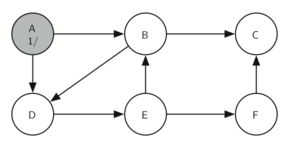
The search begins at vertex A of the graph (below). Since all of the vertices are unvisited at the beginning of the search the algorithm visits vertex A. The first step in visiting a vertex is to add it to the visited set, indicated here with a gray color, and the discovery time is set to 1. Since vertex A has two adjacent vertices (B, D) each of those need to be visited as well. We’ll make the arbitrary decision that we will visit the adjacent vertices in alphabetical order.

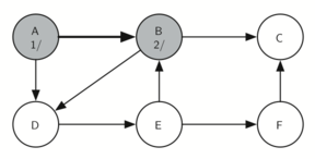
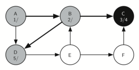
Vertex B is visited next (see below), so its color is set to gray and its discovery time is set to 2. Vertex B is also adjacent to two other nodes (C, D) so we will follow the alphabetical order and visit node C next.

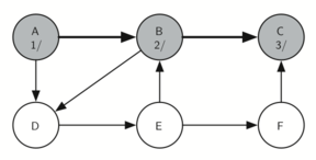
Visiting vertex C (see below) brings us to the end of one branch of the tree. After adding the node to visited and setting its discovery time to 3, the algorithm also determines that there are no adjacent vertices to C.

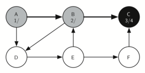
This means that we are done exploring node C and so we can color the vertex black, and set the finish time to 4. You can see the state of our search at this point below.

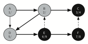
Since vertex C was the end of one branch we now return to vertex B and continue exploring the nodes adjacent to B. The only additional vertex to explore from B is D, so we can now visit D (below) and continue our search from vertex D.

Vertex D quickly leads us to vertex E:

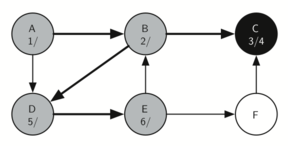
Vertex E has two adjacent vertices, B and F. Normally we would explore these adjacent vertices alphabetically, but since B has already been visited the algorithm recognizes that it should not visit B since doing so would put the algorithm in a loop! So exploration continues with the next vertex in the list, namely F.

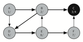
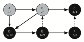
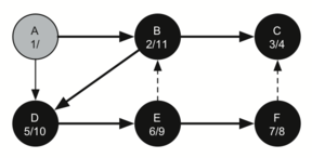
Vertex F has only one adjacent vertex, C, but since C has been visited there is nothing else to explore, and the algorithm has reached the end of another branch. From here on, you will see that the algorithm works its way back to the first node, setting finish times.

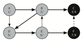
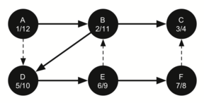
The starting and finishing times for each node display a property called the parenthesis property. This property means that all the children of a particular node in the depth first tree have a later discovery time and an earlier finish time than their parent.