Representing a Tree

In this section, we consider some different ways to represent a tree-like shape with data types in Python. It is important to become familiar with multiple representations since trees occur in many contexts and the right choice of representation in one may not quite fit another.

In Python, many of the libraries that deal with trees (such as the html5lib for parsing html, or ast for working with the abstract syntax grammar of Python) use the object oriented “nodes and references” representation we discuss first. However, when building functionality around our own trees it is generally simpler to use a representation constructed from dicts and lists, which we discuss later. This simpler representation is also more portable to other languages and contexts, even those without a notion of objects (such as pen and paper!).

Nodes and references representation

Our first method to represent a tree uses instances of a Node class along with references between node instances.

Let us consider a small example:

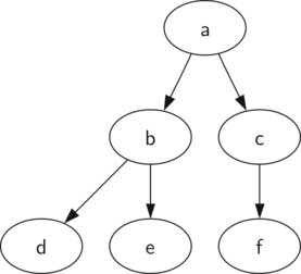
Using nodes and references, we might think of this tree as being structured like:

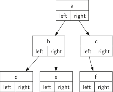
We will start out with a simple class definition for the nodes and references approach as shown below. In this case we will consider binary trees, so will directly reference left and right nodes. For trees where nodes may have more than two children, a children list could be used to contain these references instead.

The important thing to remember about this representation is that the attributes left and right will become references to other instances of the Node class. For example, when we insert a new left child into the tree we create another instance of Node and modify self.left in the root to reference the new subtree.

class Node(object):
    def __init__(self, val):
        self.val = val
        self.left = None
        self.right = None

Notice that the constructor function expects to get some kind of value to store in the node. Just like you can store any object you like in a list, the val attribute for a node can be a reference to any object. For our early examples, we will store the name of the node as the value. Using nodes and references to represent the tree illustrated above, we would create six instances of the Node class.

Next let’s look at a function that can help us build the tree beyond the root node. To add a left child to the tree, we will instantiate a new Node instance and pass it as child to the insert_left function defined here:

def insert_left(self, child):
    if self.left is None:
        self.left = child
    else:
        child.left = self.left
        self.left = child

We must consider two cases for insertion. The first case is characterized by a node with no existing left child. When there is no left child, simply add a node to the tree. The second case is characterized by a node with an existing left child. In the second case, we insert a node and push the existing child down one level in the tree.

The code for insert_right must consider a symmetric set of cases. There will either be no right child, or we must insert the node between the root and an existing right child:

def insert_right(self, child):
    if self.right is None:
        self.right = child
    else:
        child.right = self.right
        self.right = child

Now that we have all the pieces to create and manipulate a binary tree, let’s use them to check on the structure a bit more. Let’s make a simple tree with node a as the root, and add nodes b and c as children. Below we create the tree and look at the some of the values stored in key, left, and right. Notice that both the left and right children of the root are themselves distinct instances of the Node class. As we said in our original recursive definition for a tree, this allows us to treat any child of a binary tree as a binary tree itself.

root = Node('a')
root.val  # => 'a'
root.left  # => None

root.insert_left(Node('b'))
root.left  # => <__main__.Node object>
root.left.val  # => 'b'

root.insert_right(Node('c'))
root.right  # => <__main__.Node object>
root.right.val  # => 'c'

root.right.val = 'hello'
root.right.val  # => 'hello'

List of lists representation

A common way to represent trees succinctly using pure data is as a list of lists. Consider that in a list of lists, each element has one and only one parent (up to the outermost list) so meets our expectation of a tree as a hierarchical structure with no cycles.

In a list of lists tree, we will store the value of the each node as the first element of the list. The second element of the list will itself be a list that represents the left subtree. The third element of the list will be another list that represents the right subtree. To illustrate this technique, let’s consider a list of lists representation of our example tree:

tree = [
    'a',  #root
    [
        'b',  # left subtree
        ['d' [], []],
        ['e' [], []]
    ],
    [
        'c',  # right subtree
        ['f' [], []],
        []
    ]
]

Notice that we can access subtrees of the list using standard list indexing. The root of the tree is tree[0], the left subtree of the root is tree[1], and the right subtree is tree[2]. Below we illustrate creating a simple tree using a list. Once the tree is constructed, we can access the root and the left and right subtrees.

tree = ['a', ['b', ['d', [], []], ['e', [], []]], ['c', ['f', [], []], []]]

# the left subtree
tree[1]  # => ['b', ['d', [], []], ['e', [], []]]

# the right subtree
tree[2]  # => ['c', ['f', [], []], []]

# the root
tree[0]  # => 'a'

One very nice property of this list of lists approach is that the structure of a list representing a subtree adheres to the structure defined for a tree; the structure itself is recursive! A subtree that has a root value and two empty lists is a leaf node. Another nice feature of the list of lists approach is that it generalizes to a tree that has many subtrees. In the case where the tree is more than a binary tree, another subtree is just another list.

Since this representation is simply a composite of lists, we will use functions to manipulate the structure as a tree, analogous to the methods in our object oriented “nodes and references” representation above.

To add a left subtree to the root of a tree, we need to insert a new list into the second position of the root list. We must be careful. If the list already has something in the second position, we need to keep track of it and push it down the tree as the left child of the list we are adding. Here is a possible function for inserting a left child:

def insert_left(root, child_val):
    subtree = root.pop(1)
    if len(subtree) > 1:
        root.insert(1, [child_val, subtree, []])
    else:
        root.insert(1, [child_val, [], []])
    return root

Notice that to insert a left child, we first obtain the (possibly empty) list that corresponds to the current left child. We then add the new left child, installing the old left child as the left child of the new one. This allows us to splice a new node into the tree at any position. The code for insert_right is similar to insert_left and is shown below:

def insert_right(root, child_val):
    subtree = root.pop(2)
    if len(subtree) > 1:
        root.insert(2, [child_val, [], subtree])
    else:
        root.insert(2, [child_val, [], []])
    return root

To round out this set of tree-making functions, let’s write a couple of access functions for getting and setting the root value, as well as getting the left or right subtrees. This way we can abstract away the fact that we use the positions in a list to represent values, left subtrees and right subtrees:

def get_root_val(root):
    return root[0]

def set_root_val(root, new_val):
    root[0] = new_val

def get_left_child(root):
    return root[1]

def get_right_child(root):
    return root[2]

We can now use our function definitions to build a tree and retrieve children of given nodes:

root = [3, [], []]
insert_left(root, 4)
insert_left(root, 5)
insert_right(root, 6)
insert_right(root, 7)
left = get_left_child(root)
left  # => [5, [4, [], []], []]

set_root_val(left, 9)
root  # => [3, [9, [4, [], []], []], [7, [], [6, [], []]]]

insert_left(left, 11)
root  # => [3, [9, [11, [4, [], []], []], []], [7, [], [6, [], []]]]
get_right_child(get_right_child(root))  # => [6, [], []]

Map-based representation

Our list of list representation has a handful of benefits:

1. It is succinct;
2. We can easily construct the tree as Python list literals;
3. We can easily serialize and print the tree; and,
4. It is portable to languages and contexts without objects.

However, it has the significant disadvantage that it is somewhat difficult to see the tree-like nature of the composite lists simply by looking at one, particularly if it is printed on a single line.

For this reason, our preference in this book (and often in real-life programming, for that matter) is to use a very similar representation using nested mappings (i.e. of dicts in Python) such that we can name children, values and potentially other data related to a tree node.

Using maps, our example tree may look like:

{
    'val': 'A',
    'left': {
        'val': 'B',
        'left': {'val': 'D'},
        'right': {'val': 'E'}
    },
    'right': {
        'val': 'C',
        'right': {'val': 'F'}
    }
}

In this case, each of our nodes becomes a map with at least the val key, and in some cases a left and/or right key(s).

If we were dealing with a tree that is not a binary tree, we could use a children key instead:

{
    'val': 'A',
    'children': [
        {
            'val': 'B',
            'children': [
                {'val': 'D'},
                {'val': 'E'},
            ]
        },
        {
            'val': 'C',
            'children': [
                {'val': 'F'},
                {'val': 'G'},
                {'val': 'H'}
            ]
        }
    ]
}

This is almost as compact as our list of lists representation, and significantly more readable, so we will continue to use this map-based representation throughout the book.