A Knight’s Tour

The “knight’s tour” is a classic problem in graph theory, first posed over 1,000 years ago and pondered by legendary mathematicians including Leonhard Euler before finally being solved in 1823. We will use the knight’s tour problem to illustrate a second common graph algorithm called depth first search.

The knight’s tour puzzle is played on a chess board with a single chess piece, the knight. The object of the puzzle is to find a sequence of moves that allow the knight to visit every square on the board exactly once, like so:

One such sequence is called a “tour.” The upper bound on the number of possible legal tours for an eight-by-eight chessboard is known to be $1.305 \times 10^{35}$; however, there are even more possible dead ends. Clearly this is a problem that requires some real brains, some real computing power, or both.

Once again we will solve the problem using two main steps:

• Represent the legal moves of a knight on a chessboard as a graph.
• Use a graph algorithm to find a path where every vertex on the graph is visited exactly once.

Building the Knight’s Tour Graph

To represent the knight’s tour problem as a graph we will use the following two ideas: Each square on the chessboard can be represented as a node in the graph. Each legal move by the knight can be represented as an edge in the graph.

We will use a Python dictionary to hold our graph, with the keys being tuples of coordinates representing the squares of the board, and the values being sets representing the valid squares to which a knight can move from that square.

To build the full graph for an n-by-n board we can use the Python function shown below. The build_graph function makes one pass over the entire board. At each square on the board the build_graph function calls a helper generator, legal_moves_from, to generate a list of legal moves for that position on the board. All legal moves are then made into undirected edges of the graph by adding the vertices appropriately to one anothers sets of legal moves.

from collections import defaultdict


def add_edge(graph, vertex_a, vertex_b):
    graph[vertex_a].add(vertex_b)
    graph[vertex_b].add(vertex_a)


def build_graph(board_size):
    graph = defaultdict(set)
    for row in range(board_size):
        for col in range(board_size):
            for to_row, to_col in legal_moves_from(row, col, board_size):
                add_edge(graph, (row, col), (to_row, to_col))
    return graph

The legal_moves_from generator below takes the position of the knight on the board and yields any of the eight possible moves that are still on the board.

MOVE_OFFSETS = (
              (-1, -2), ( 1, -2),
    (-2, -1),                     ( 2, -1),
    (-2,  1),                     ( 2,  1),
              (-1,  2), ( 1,  2),
)


def legal_moves_from(row, col, board_size):
    for row_offset, col_offset in MOVE_OFFSETS:
        move_row, move_col = row + row_offset, col + col_offset
        if 0 <= move_row < board_size and 0 <= move_col < board_size:
            yield move_row, move_col

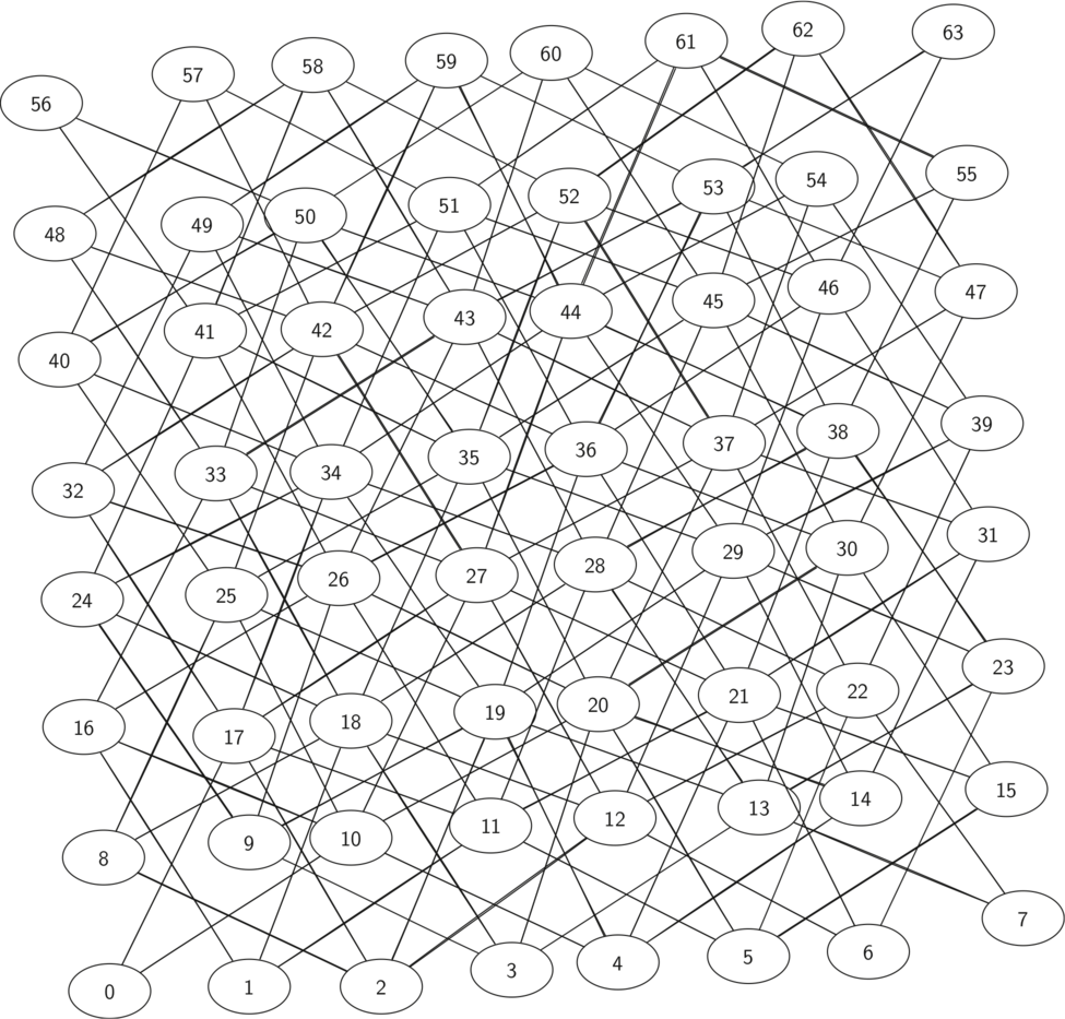
The illustration below shows the complete graph of possible moves on an eight-by-eight board. There are exactly 336 edges in the graph. Notice that the vertices corresponding to the edges of the board have fewer connections (legal moves) than the vertices in the middle of the board. Once again we can see how sparse the graph is. If the graph was fully connected there would be 4,096 edges. Since there are only 336 edges, the adjacency matrix would be only 8.2 percent full.

Implementing Knight’s Tour

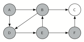
The search algorithm we will use to solve the knight’s tour problem is called depth first search (DFS). Whereas the breadth first search algorithm discussed in the previous section builds a search tree one level at a time, a depth first search creates a search tree by exploring one branch of the tree as deeply as possible.

The depth first exploration of the graph is exactly what we need in order to find a path that has exactly 63 edges. We will see that when the depth first search algorithm finds a dead end (a place in the graph where there are no more moves possible) it backs up the tree to the next deepest vertex that allows it to make a legal move.

The find_solution_for function takes just two arguments: a board_size argument and a heuristic function, which you should ignore for now but to which we will return.

It then constructs a graph using the build_graph function described above, and for each vertex in the graph attempts to traverse depth first by way of the traverse function.

The traverse function is a little more interesting. It accepts a path, as a list of coordinates, as well as the vertex currently being considered. If the traversal has proceeded deep enough that we know that every square has been visited once, then we return the full path traversed.

Otherwise, we use our graph to look up the legal moves from the current vertex, and exclude the vertices that we know have already been visited, to determine the vertices that are yet_to_visit. At this point we recursively call traverse with each of the vertices to visit, along with the path to reach that vertex including the current vertex. If any of the recursive calls return a path, then that path is the return value of the outer call, otherwise we return None.

def first_true(sequence):
    for item in sequence:
        if item:
            return item
    return None


def find_solution_for(board_size, heuristic=lambda graph: None):
    graph = build_graph(board_size)
    total_squares = board_size * board_size

    def traverse(path, current_vertex):
        if len(path) + 1 == total_squares:
            # including the current square, we've visited every square,
            # so return the path as a solution
            return path + [current_vertex]

        yet_to_visit = graph[current_vertex] - set(path)
        if not yet_to_visit:
            # no unvisited neighbors, so dead end
            return False

        # try all valid paths from here
        next_vertices = sorted(yet_to_visit, heuristic(graph))
        return first_true(traverse(path + [current_vertex], vertex)
                          for vertex in next_vertices)

    # try to find a solution from any square on the board
    return first_true(traverse([], starting_vertex)
                      for starting_vertex in graph)


# find_solution_for(5)  # => [(1, 3), (0, 1), (2, 0), (4, 1), (2, 2), ... ]

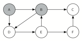
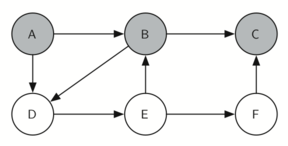
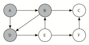
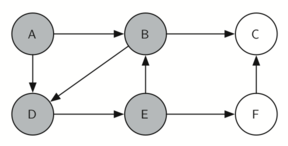
Let’s look at a simple example of an equivalent of this traverse function in action.

It is remarkable that our choice of data structure and algorithm has allowed us to straightforwardly solve a problem that remained impervious to thoughtful mathematical investigation for centuries.

With some modification, the algorithm can also be used to discover one of a number of “closed” (circular) tours, which can therefore be started at any square of the board:

Knight’s Tour Analysis

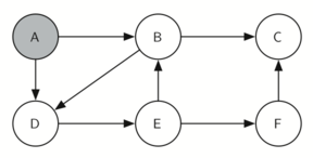
There is one last interesting topic regarding the knight’s tour problem, then we will move on to the general version of the depth first search. The topic is performance. In particular, our algorithm is very sensitive to the method you use to select the next vertex to visit. For example, on a five-by-five board you can produce a path in about 1.5 seconds on a reasonably fast computer. But what happens if you try an eight-by-eight board? In this case, depending on the speed of your computer, you may have to wait up to a half hour to get the results! The reason for this is that the knight’s tour problem as we have implemented it so far is an exponential algorithm of size $O(k^N)$, where N is the number of squares on the chess board, and k is a small constant. The diagram below can help us visualize why this is so.

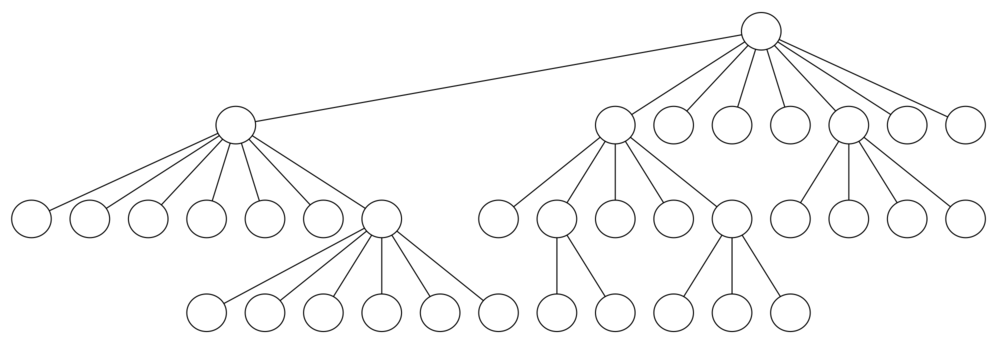
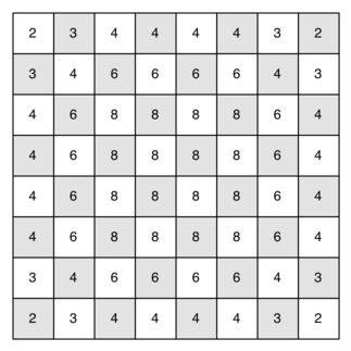
The root of the tree represents the starting point of the search. From there the algorithm generates and checks each of the possible moves the knight can make. As we have noted before the number of moves possible depends on the position of the knight on the board. In the corners there are only two legal moves, on the squares adjacent to the corners there are three and in the middle of the board there are eight. The diagram below shows the number of moves possible for each position on a board. At the next level of the tree there are once again between 2 and 8 possible next moves from the position we are currently exploring. The number of possible positions to examine corresponds to the number of nodes in the search tree.

We have already seen that the number of nodes in a binary tree of height N is $2^{N+1}-1$. For a tree with nodes that may have up to eight children instead of two the number of nodes is much larger. Because the branching factor of each node is variable, we could estimate the number of nodes using an average branching factor. The important thing to note is that this algorithm is exponential: $k^{N+1}-1$, where $k$ is the average branching factor for the board. Let’s look at how rapidly this grows! For a board that is 5x5 the tree will be 25 levels deep, or N = 24 counting the first level as level 0. The average branching factor is $k = 3.8$ So the number of nodes in the search tree is $3.8^{25}-1$ or $3.12 \times 10^{14}$. For a 6x6 board, $k = 4.4$, there are $1.5 \times 10^{23}$ nodes, and for a regular 8x8 chess board, $k = 5.25$, there are $1.3 \times 10^{46}$. Of course, since there are multiple solutions to the problem we won’t have to explore every single node, but the fractional part of the nodes we do have to explore is just a constant multiplier which does not change the exponential nature of the problem. We will leave it as an exercise for you to see if you can express $k$ as a function of the board size.

Luckily there is a way to speed up the eight-by-eight case so that it runs in under one second. In the code sample below we show the code that speeds up the traverse. This function, called warnsdorffs_heuristic when passed as the heuristic function to find_solution_for above will cause the next_vertices to be sorted prioritizing those who which have the fewest subsequent legal moves.

This may seem counterintutitive; why not select the node that has the most available moves? The problem with using the vertex with the most available moves as your next vertex on the path is that it tends to have the knight visit the middle squares early on in the tour. When this happens it is easy for the knight to get stranded on one side of the board where it cannot reach unvisited squares on the other side of the board. On the other hand, visiting the squares with the fewest available moves first pushes the knight to visit the squares around the edges of the board first. This ensures that the knight will visit the hard-to- reach corners early and can use the middle squares to hop across the board only when necessary. Utilizing this kind of knowledge to speed up an algorithm is called a heuristic. Humans use heuristics every day to help make decisions, heuristic searches are often used in the field of artificial intelligence. This particular heuristic is called Warnsdorff’s heuristic, named after H. C. Warnsdorff who published his idea in 1823, becoming the first person to describe a procedure to complete the knight’s tour.

def warnsdorffs_heuristic(graph):

    #Given a graph, return a comparator function that prioritizes nodes
    #with the fewest subsequent moves
    def comparator(a, b):
        return len(graph[a]) - len(graph[b])

    return comparator

# find_solution_for(8, warnsdorffs_heuristic)
# => [(7, 3), (6, 1), (4, 0), (2, 1), (0, 0), (1, 2), ... ]

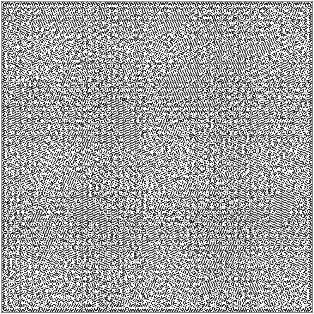
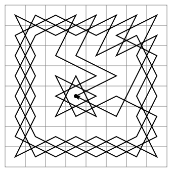
For fun, here is a very large ($130 \times 130$) open knight’s tour created using Warnsdorff’s heuristic: