The Binary Search
It is possible to take greater advantage of the ordered list if we are clever with our comparisons. In the sequential search, when we compare against the first item, there are at most more items to look through if the first item is not what we are looking for. Instead of searching the list in sequence, a binary search will start by examining the middle item. If that item is the one we are searching for, we are done. If it is not the correct item, we can use the ordered nature of the list to eliminate half of the remaining items. If the item we are searching for is greater than the middle item, we know that the entire lower half of the list as well as the middle item can be eliminated from further consideration. The item, if it is in the list, must be in the upper half.
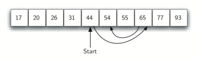
We can then repeat the process with the upper half. Start at the middle item and compare it against what we are looking for. Again, we either find it or split the list in half, therefore eliminating another large part of our possible search space. The diagram below shows how this algorithm can quickly find the value 54.
This algorithm is a great example of a divide and conquer strategy. Divide and conquer means that we divide the problem into smaller pieces, solve the smaller pieces in some way, and then reassemble the whole problem to get the result. When we perform a binary search of a list, we first check the middle item. If the item we are searching for is less than the middle item, we can simply perform a binary search of the left half of the original list. Likewise, if the item is greater, we can perform a binary search of the right half. Either way, this is a recursive call to the binary search function passing a smaller list.
An implementation of recursive binary search in Python may look like this:
def binary_search(alist, item):
    if not alist:  # list is empty -- our base case
        return False

    midpoint = len(alist) // 2
    if alist[midpoint] == item:  # found it!
        return True

    if item < alist[midpoint]:  # item is in the first half, if at all
        return binary_search(alist[:midpoint], item)

    # otherwise item is in the second half, if at all
    return binary_search(alist[midpoint + 1:], item)


testlist = [0, 1, 2, 8, 13, 17, 19, 32, 42]
binary_search(testlist, 3)  # => False
binary_search(testlist, 13)  # => True
Analysis of Binary Search
To analyze the binary search algorithm, we need to recall that each comparison eliminates around half of the remaining items from consideration. What is the maximum number of comparisons this algorithm will require to check the entire list? If we start with n items, approximately items will be left after the first comparison. After the second comparison, there will be approximately . Then , , and so on. How many times can we split the list? This table helps us to see the answer:
| Comparisons | Approximate Number of Items Left |
|---|---|
| 1 | |
| 2 | |
| 3 | |
| ... | |
| i |
When we split the list enough times, we end up with a list that has just one item. Either that is the item we are looking for or it is not. Either way, we are done. The number of comparisons necessary to get to this point is i where . Solving for i gives us . The maximum number of comparisons is logarithmic with respect to the number of items in the list. Therefore, the binary search is .
One additional analysis issue needs to be addressed. In the solution shown above, the recursive call,
binary_search(alist[:midpoint], item)
uses the slice operator to create the left half of the list that is then passed to the next invocation (similarly for the right half as well). The analysis that we did above assumed that the slice operator takes constant time. However, we know that the slice operator in Python is actually . This means that the binary search using slice will not perform in strict logarithmic time. Luckily this can be remedied by passing the list along with the starting and ending indices. We leave this implementation as an exercise.
Even though a binary search is generally better than a sequential search, it is important to note that for small values of n, the additional cost of sorting is probably not worth it. In fact, we should always consider whether it is cost effective to take on the extra work of sorting to gain searching benefits. If we can sort once and then search many times, the cost of the sort is not so significant. However, for large lists, sorting even once can be so expensive that simply performing a sequential search from the start may be the best choice.