Word Ladders

To begin our study of graph algorithms let’s consider the following puzzle called a word ladder. Transform the word “FOOL” into the word “SAGE”. In a word ladder puzzle you must make the change occur gradually by changing one letter at a time. At each step you must transform one word into another word, you are not allowed to transform a word into a non-word. The word ladder puzzle was invented in 1878 by Lewis Carroll, the author of Alice in Wonderland. The following sequence of words shows one possible solution to the problem posed above.

FOOL
POOL
POLL
POLE
PALE
SALE
SAGE

There are many variations of the word ladder puzzle. For example you might be given a particular number of steps in which to accomplish the transformation, or you might need to use a particular word. In this section we are interested in figuring out the smallest number of transformations needed to turn the starting word into the ending word.

Not surprisingly, since this chapter is on graphs, we can solve this problem using a graph algorithm. Here is an outline of where we are going:

• Represent the relationships between the words as a graph.
• Use the graph algorithm known as breadth first search to find an efficient path from the starting word to the ending word.

Building the Word Ladder Graph

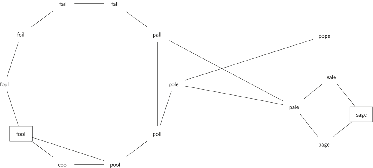
Our first problem is to figure out how to turn a large collection of words into a graph. What we would like is to have an edge from one word to another if the two words are only different by a single letter. If we can create such a graph, then any path from one word to another is a solution to the word ladder puzzle. The illustration below shows a small graph of some words that solve the FOOL to SAGE word ladder problem. Notice that the graph is an undirected graph and that the edges are unweighted.

We could use several different approaches to create the graph we need to solve this problem. Let’s start with the assumption that we have a list of words that are all the same length. As a starting point, we can create a vertex in the graph for every word in the list. To figure out how to connect the words, we could compare each word in the list with every other. When we compare we are looking to see how many letters are different. If the two words in question are different by only one letter, we can create an edge between them in the graph. For a small set of words that approach would work fine; however let’s suppose we have a list of 5,110 words. Roughly speaking, comparing one word to every other word on the list is an $O(n^2)$ algorithm. For 5,110 words, $n^2$ is more than 26 million comparisons.

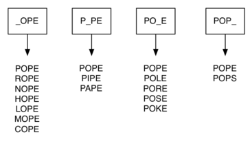
We can do much better by using the following approach. Suppose that we have a huge number of buckets, each of them with a four-letter word on the outside, except that one of the letters in the label has been replaced by an underscore. For example we might have a bucket labeled “pop_.” As we process each word in our list we compare the word with each bucket, using the ‘_’ as a wildcard, so both “pope” and “pops” would match “pop_.” Every time we find a matching bucket, we put our word in that bucket. Once we have all the words in the appropriate buckets we know that all the words in the bucket must be connected.

In Python, we can implement the scheme we have just described by using a dictionary. The labels on the buckets we have just described are the keys in our dictionary. The value stored for that key is a list of words. Once we have the dictionary built we can create the graph. We start our graph by creating a vertex for each word in the graph. Then we create edges between all the vertices we find for words found under the same key in the dictionary.

Below is an example of Python code implementing this strategy. In this case, we use a dictionary mapping vertices (words) to sets of the vertices that can be reached by changing one letter in that word.

from collections import defaultdict
from itertools import product
import os


def build_graph(words):
    buckets = defaultdict(list)
    graph = defaultdict(set)

    for word in words:
        for i in range(len(word)):
            bucket = '{}_{}'.format(word[:i], word[i + 1:])
            buckets[bucket].append(word)

    # add vertices and edges for words in the same bucket
    for bucket, mutual_neighbors in buckets.items():
        for word1, word2 in product(mutual_neighbors, repeat=2):
            if word1 != word2:
                graph[word1].add(word2)
                graph[word2].add(word1)

    return graph


def get_words(vocabulary_file):
    for line in open(vocabulary_file, 'r'):
        yield line[:-1]  # remove newline character


vocabulary_file = os.path.join(os.path.dirname(__file__), 'vocabulary.txt')
word_graph = build_graph(get_words(vocabulary_file))

# word_graph['FOOL']
# set(['POOL', 'WOOL', 'FOWL', 'FOAL', 'FOUL', ... ])

Since this is our first real-world graph problem, you might be wondering how sparse is the graph? The list of four-letter words we have for this problem is 5,110 words long. If we were to use an adjacency matrix, the matrix would have 5,110 * 5,110 = 26,112,100 cells. The graph constructed by the build_graph function has exactly 53,286 edges, so the matrix would have only 0.20% of the cells filled! That is a very sparse matrix indeed.

Implementing breadth first search

With the graph constructed we can now turn our attention to the algorithm we will use to find the shortest solution to the word ladder problem. The graph algorithm we are going to use is called the “breadth first search” algorithm. Breadth first search (BFS) is one of the easiest algorithms for searching a graph. It also serves as a prototype for several other important graph algorithms that we will study later.

Given a graph $G$ and a starting vertex $s$, a breadth first search proceeds by exploring edges in the graph to find all the vertices in $G$ for which there is a path from $s$. The remarkable thing about a breadth first search is that it finds all the vertices that are a distance $k$ from $s$ before it finds any vertices that are a distance $k+1$. One good way to visualize what the breadth first search algorithm does is to imagine that it is building a tree, one level of the tree at a time. A breadth first search adds all children of the starting vertex before it begins to discover any of the grandchildren.

The breadth first search algorithm shown below uses the adjacency list graph representation we developed earlier. In addition it uses a queue at a crucial point as we will see, to decide which vertex to explore next, and also to maintain a record of the depth to which we have traversed at any point.

BFS starts by initializing a set to retain a record of which vertices have been visited already. Next, we initialize a queue (in this case utilizing the deque type from Python’s collections module) which will contain all paths from our starting vertex that we have explored as our algorithm progress. As such we initialize it with a list containing just our starting vertex.

The next step is to begin to systematically grow the paths one at a time, starting from the path at the front of the queue, in each case taking one more step from the vertex last explored.

Once we have popped from our queue a path to continue exploring and retrieved the last the vertex visited from that path, we retrieve its neighbors from our graph, remove those vertices that we know have already been visited, then for each of the remaining (unvisited) neighbors do two things:

1. Add the vertex to visited
2. Add a path consisisting of the path so far plus the vertex

Adding the new vertex effectively schedules it for further exploration, but not until all the other vertices on the adjacency list have been explored.

from collections import deque


def traverse(graph, starting_vertex):
    visited = set()
    queue = deque([[starting_vertex]])
    while queue:
        path = queue.popleft()
        vertex = path[-1]
        yield vertex, path
        for neighbor in graph[vertex] - visited:
            visited.add(neighbor)
            queue.append(path + [neighbor])

if __name__ == '__main__':
    for vertex, path in traverse(word_graph, 'FOOL'):
        if vertex == 'SAGE':
            print ' -> '.join(path)
            # FOOL -> FOOD -> FOLD -> SOLD -> SOLE -> SALE -> SAGE

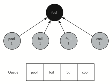
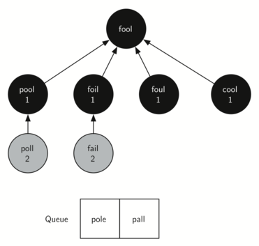
Let’s look at how the traverse function would construct the breadth first tree corresponding to the word ladder graph we considered previously. Starting from fool we take all nodes that are adjacent to fool and add them to the tree. The adjacent nodes include pool, foil, foul, and cool. Each of these nodes are added to the queue of new nodes to expand. The illustration below shows the state of the in-progress tree along with the queue after this step.

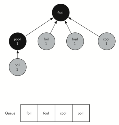
In the next step traverse removes the next node (pool) from the front of the queue and repeats the process for all of its adjacent nodes. However, when traverse examines the node cool, it finds that it has already been visited. This implies that there is a shorter path to cool. The only new node added to the queue while examining pool is poll. The new state of the tree and queue is shown below.

The next vertex on the queue is foil. The only new node that foil can add to the tree is fail. As traverse continues to process the queue, neither of the next two nodes add anything new to the queue or the tree. The illustration below shows the tree and the queue after expanding all the vertices on the second level of the tree.

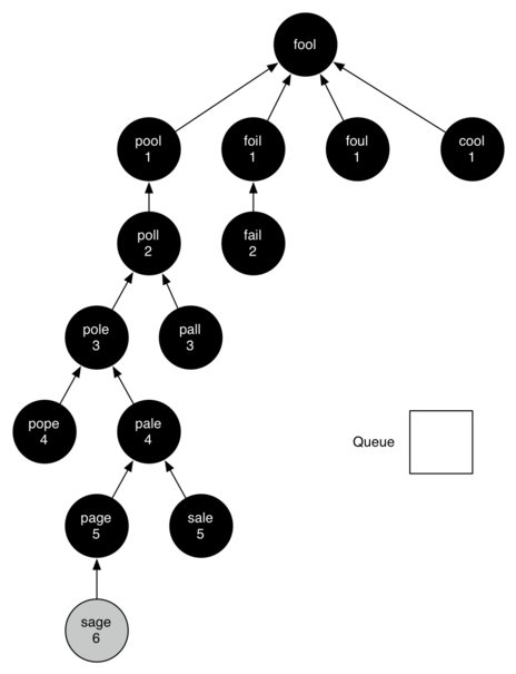
You should continue to work through the algorithm on your own so that you are comfortable with how it works. The illustration below shows the final breadth first search tree after all the vertices have been expanded.

Breadth First Search Analysis

Before we continue with other graph algorithms let us analyze the run time performance of the breadth first search algorithm. The first thing to observe is that the while loop is executed, at most, one time for each vertex in the graph $|V|$. You can see that this is true because a vertex must be white before it can be examined and added to the queue. This gives us $O(V)$ for the while loop. The for loop, which is nested inside the while is executed at most once for each edge in the graph, $|E|$. The reason is that every vertex is dequeued at most once and we examine an edge from node $u$ to node $v$ only when node $u$ is dequeued. This gives us $O(E)$ for the for loop. combining the two loops gives us $O(V + E)$.

Of course doing the breadth first search is only part of the task. Following the links from the starting node to the goal node is the other part of the task. The worst case for this would be if the graph was a single long chain. In this case traversing through all of the vertices would be $O(V)$. The normal case is going to be some fraction of $|V|$ but we would still write $O(V)$.

Finally, at least for this problem, there is the time required to build the initial graph. We leave the analysis of the build_graph function as an exercise for you.