Shortest Path with Dijkstra’s Algorithm

When you surf the web, send an email, or log in to a laboratory computer from another location on campus a lot of work is going on behind the scenes to get the information on your computer transferred to another computer. The in-depth study of how information flows from one computer to another over the Internet is the primary topic for a class in computer networking. However, we will talk about how the Internet works just enough to understand another very important graph algorithm.

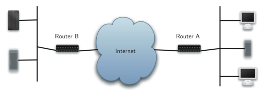
The diagram above shows you a high-level overview of how communication on the Internet works. When you use your browser to request a web page from a server, the request must travel over your local area network and out onto the Internet through a router. The request travels over the Internet and eventually arrives at a router for the local area network where the server is located. The web page you requested then travels back through the same routers to get to your browser. Inside the cloud labeled “Internet” in the diagram are additional routers. The job of all of these routers is to work together to get your information from place to place. You can see there are many routers for yourself if your computer supports the traceroute command. The text below shows the output of running traceroute google.com on the author’s computer, which illustrates that there are 12 routers between him and the Google server responding to the request.

traceroute to google.com (216.58.192.46), 64 hops max, 52 byte packets
 1  192.168.0.1 (192.168.0.1)  3.420 ms  1.133 ms  0.865 ms
 2  gw-mosca207.static.monkeybrains.net (199.188.195.1)  14.678 ms  9.725 ms  6.752 ms
 3  mosca.mosca-activspace.core.monkeybrains.net (172.17.18.58)  8.919 ms  8.277 ms  7.804 ms
 4  lemon.lemon-mosca-10gb.core.monkeybrains.net (208.69.43.185)  6.724 ms  7.369 ms  6.701 ms
 5  38.88.216.117 (38.88.216.117)  8.420 ms  11.860 ms  6.813 ms
 6  be2682.ccr22.sfo01.atlas.cogentco.com (154.54.6.169)  7.392 ms  7.250 ms  8.241 ms
 7  be2164.ccr21.sjc01.atlas.cogentco.com (154.54.28.34)  8.710 ms  8.301 ms  8.501 ms
 8  be2000.ccr21.sjc03.atlas.cogentco.com (154.54.6.106)  9.072 ms
    be2047.ccr21.sjc03.atlas.cogentco.com (154.54.5.114)  11.034 ms
    be2000.ccr21.sjc03.atlas.cogentco.com (154.54.6.106)  10.243 ms
 9  38.88.224.6 (38.88.224.6)  8.420 ms  10.637 ms  8.855 ms
10  209.85.249.5 (209.85.249.5)  9.142 ms  17.734 ms  12.211 ms
11  74.125.37.43 (74.125.37.43)  8.792 ms  9.290 ms  8.893 ms
12  nuq04s30-in-f14.1e100.net (216.58.192.46)  8.759 ms  8.705 ms  8.502 ms

Each router on the Internet is connected to one or more other routers. So if you run the traceroute command at different times of the day, you are likely to see that your information flows through different routers at different times. This is because there is a cost associated with each connection between a pair of routers that depends on the volume of traffic, the time of day, and many other factors. By this time it will not surprise you to learn that we can represent the network of routers as a graph with weighted edges.

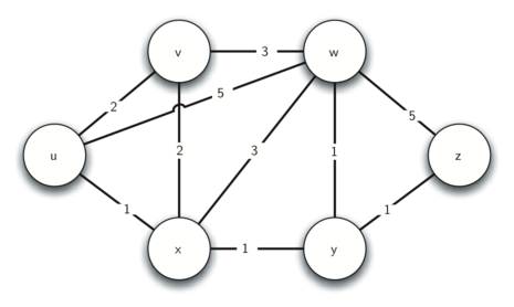
Above we show a small example of a weighted graph that represents the interconnection of routers in the Internet. The problem that we want to solve is to find the path with the smallest total weight along which to route any given message. This problem should sound familiar because it is similar to the problem we solved using a breadth first search, except that here we are concerned with the total weight of the path rather than the number of hops in the path. It should be noted that if all the weights are equal, the problem is the same.

Dijkstra’s Algorithm

The algorithm we are going to use to determine the shortest path is called “Dijkstra’s algorithm.” Dijkstra’s algorithm is an iterative algorithm that provides us with the shortest path from one particular starting node to all other nodes in the graph. Again this is similar to the results of a breadth first search.

To keep track of the total cost from the start node to each destination we will make use of a distances dictionary which we will initialize to 0 for the start vertex, and infinity for the other vertices. Our algorithm will update these values until they represent the smallest weight path from the start to the vertex in question, at which point we will return the distances dictionary.

The algorithm iterates once for every vertex in the graph; however, the order that we iterate over the vertices is controlled by a priority queue. The value that is used to determine the order of the objects in the priority queue is the distance from our starting vertex. By using a priority queue, we ensure that as we explore one vertex after another, we are always exploring the one with the smallest distance.

The code for Dijkstra’s algorithm is shown below.

import heapq


def calculate_distances(graph, starting_vertex):
    distances = {vertex: float('infinity') for vertex in graph}
    distances[starting_vertex] = 0

    pq = [(0, starting_vertex)]
    while len(pq) > 0:
        current_distance, current_vertex = heapq.heappop(pq)

        # Nodes can get added to the priority queue multiple times. We only
        # process a vertex the first time we remove it from the priority queue.
        if current_distance > distances[current_vertex]:
            continue

        for neighbor, weight in graph[current_vertex].items():
            distance = current_distance + weight

            # Only consider this new path if it's better than any path we've
            # already found.
            if distance < distances[neighbor]:
                distances[neighbor] = distance
                heapq.heappush(pq, (distance, neighbor))

    return distances


example_graph = {
    'U': {'V': 2, 'W': 5, 'X': 1},
    'V': {'U': 2, 'X': 2, 'W': 3},
    'W': {'V': 3, 'U': 5, 'X': 3, 'Y': 1, 'Z': 5},
    'X': {'U': 1, 'V': 2, 'W': 3, 'Y': 1},
    'Y': {'X': 1, 'W': 1, 'Z': 1},
    'Z': {'W': 5, 'Y': 1},
}
print(calculate_distances(example_graph, 'X'))
# => {'U': 1, 'W': 2, 'V': 2, 'Y': 1, 'X': 0, 'Z': 2}

Dijkstra’s algorithm uses a priority queue, which we introduced in the trees chapter and which we achieve here using Python’s heapq module.

The entries in our priority queue are tuples of (distance, vertex) which allows us to maintain a queue of vertices sorted by distance.

When the distance to a vertex that is already in the queue is reduced, we wish to update the distance and thereby give it a different priority. We accomplish this by just adding another entry to the priority queue for the same vertex. (We also include a check after removing an entry from the priority queue, in order to make sure that we only process each vertex once.)

Let’s walk through an application of Dijkstra’s algorithm one vertex at a time using the following sequence of diagrams as our guide. We begin with the vertex $u$. The three vertices adjacent to $u$ are $v,w,$ and $x$. Since the initial distances to $v,w,$ and $x$ are all initialized to infinity, the new costs to get to them through the start node are all their direct costs. So we update the costs to each of these three nodes. The state of the algorithm is:

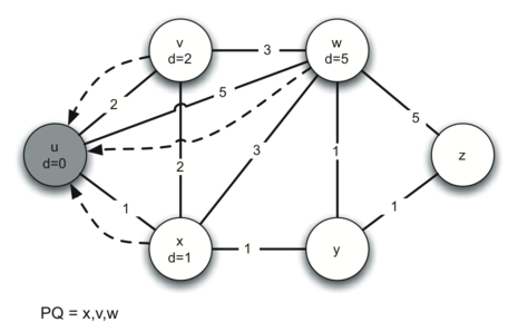
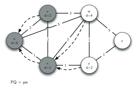
In the next iteration of the while loop we examine the vertices that are adjacent to $u$. The vertex $x$ is next because it has the lowest overall cost and therefore will be the first entry removed from the priority queue. At $x$ we look at its neighbors $u,v,w$ and $y$. For each neighboring vertex we check to see if the distance to that vertex through $x$ is smaller than the previously known distance. Obviously this is the case for $y$ since its distance was infinity. It is not the case for $u$ or $v$ since their distances are 0 and 2 respectively. However, we now learn that the distance to $w$ is smaller if we go through $x$ than from $u$ directly to $w$. Since that is the case we update $w$ with a new distance and add another entry to the priority queue. The state of the algorithm is now:

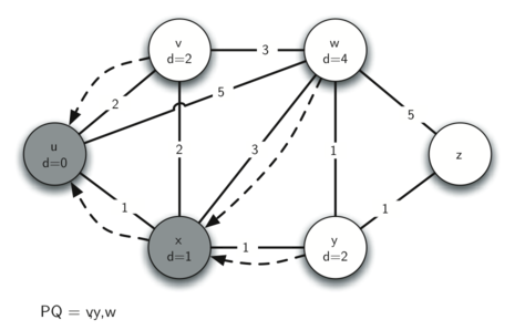
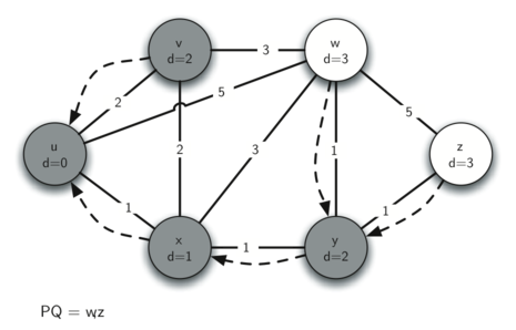
The next step is to look at the vertices neighboring $v$ (below). This step results in no changes to the graph, so we move on to node $y$.

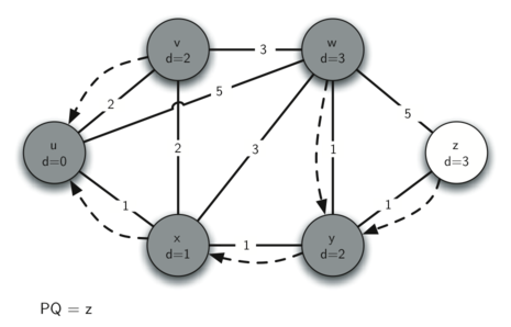
At node $y$ (below) we discover that it is cheaper to get to both $w$ and $z$, so we adjust the distances accordingly.

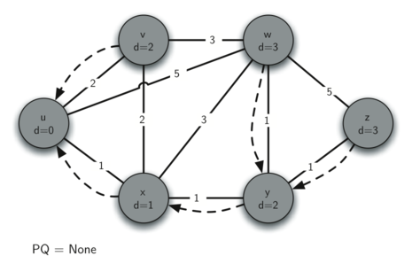
Finally we check nodes $w$ and $z$. However, no additional changes are found and so the priority queue is empty and Dijkstra’s algorithm exits.

It is important to note that Dijkstra’s algorithm works only when the weights are all positive. You should convince yourself that if you introduced a negative weight on one of the edges to the graph that the algorithm would never exit.

We will note that to route messages through the Internet, other algorithms are used for finding the shortest path. One of the problems with using Dijkstra’s algorithm on the Internet is that you must have a complete representation of the graph in order for the algorithm to run. The implication of this is that every router has a complete map of all the routers in the Internet. In practice this is not the case and other variations of the algorithm allow each router to discover the graph as they go. One such algorithm that you may want to read about is called the “distance vector” routing algorithm.

Analysis of Dijkstra’s Algorithm

We will now consider the running time of Dijkstra’s algorithm.

Building the distances dictionary takes $O(V)$ time since we add every vertex in the graph to the dictionary.

The while loop is executed once for every entry that gets added to the priority queue. An entry can only be added when we explore an edge, so there are at most $O(E)$ iterations of the while loop.

The for loop is executed at most once for every vertex, since the current_distance > distances[current_vertex] check ensures that we only process a vertex once. The for loop iterates over outgoing edges, so among all iterations of the while loop, the body of the for loop executes at most $O(E)$ times.

Finally, if we consider that each priority queue operation (adding or removing an entry) is $O(\log E)$, we conclude that the total running time is $O(V + E \log E)$.